Linear Regression

What is Regression?And Linear Regression

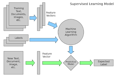
A statistical measure that attempts to determine the strength of the relationship between one dependent variable (usually denoted by Y) and a series of other changing variables (known as independent variables). Regression is very powerful technique for prediction in Machine Learning. Regression is Supervised Learning type algorithm.

 

Different types of Regression:

• Linear Regression
• Logistic Regression 

Linear Regression:

In simple linear regression, we predict scores on one variable from the scores on a second variable. The variable we are predicting is called the criterion variable and is referred to as Y. The variable we are basing our predictions on is called the predictor variable and is referred to as X. When there is only one predictor variable, the prediction method is called simple regression. In simple linear regression, the topic of this section, the predictions of Y when plotted as a function of X form a straight line.

A linear regression line has an equation of the form Y = a + bX, where X is the explanatory variable and Y is the dependent variable. The slope of the line is b, and a is the intercept (the value of y when x = 0).

Suppose, data about Temperature is as given below in Table - 1

 Table - 1

 We can obtain scatter plot of given data in Table - 1 in Cartesian coordinate system as show in Plot - 1,

Plot - 1

It is clear that no line can be found to pass through all points of the plot. Thus no functional relation exists between the two variables x and Y. However, the scatter plot does give an indication that a straight line may exist such that all the points on the plot are scattered randomly around this line. A statistical relation is said to exist in this case. The statistical relation between x and Y may be expressed as follows: 

Y =  B0 + B1*x + e

The above equation is the linear regression model that can be used to explain the relation between x and Y that is seen on the scatter plot above. In this model, the mean value of Y (abbreviated as E(Y)) is assumed to follow the linear relation:

E(Y) = B0 + B1*x

The actual values of Y (which are observed as yield from the chemical process from time to time and are random in nature) are assumed to be the sum of the mean value, E(Y), and a random error term, e: 

Y = E(Y)  + e
   = B0 + B1*x + e

The regression model here is called a simple linear regression model because there is just one independent variable, x, in the model. In regression models, the independent variables are also referred to as regressors or predictor variables. The dependent variable, Y , is also referred to as the response. The slope, B1, and the intercept, B0 , of the line E(Y) = B0 + B1*x are called regression coefficients. The slope, B1, can be interpreted as the change in the mean value of Y for a unit change in x.

Plot - 2

Fitted Regression Line

The true regression line is usually not known. However, the regression line can be estimated by estimating the coefficients and for an observed data set. The estimates, and , are calculated using least squares. The estimated regression line, obtained using the values of and , is called the fitted line. The least square estimates, and , are obtained using the following equations:

where is the mean of all the observed values and is the mean of all values of the predictor variable at which the observations were taken. is calculated using and is calculated using .

Once and are known, the fitted regression line can be written as:

where is the fitted or estimated value based on the fitted regression model. It is an estimate of the mean value, . The fitted value,, for a given value of the predictor variable, , may be different from the corresponding observed value, . The difference between the two values is called the residual, :

Calculation of the Fitted Line Using Least Square Estimates

The least square estimates of the regression coefficients can be obtained for the data in the preceding Table - 1 as follows:

Knowing both the coefficient ,the fitted regression line is: 

This line is shown in the Plot - 3 below. 

Plot - 3

Now, we can predict value of Y for any given value of x by just putting the value of x in Regression Line.

Introduction To Supervised Learning

What is Supervised Learning?

Introduction

Supervised Learning is the Machine Learning task of inferring a function from labelled training data. The training data consist of a set of training examples. In supervised learning, each example is a pair consisting of an input object (typically a vector) and a desired output value (also called the supervisory signal). A supervised learning algorithm analyses the training data and produces an inferred function, which can be used for mapping new examples. An optimal scenario will allow for the algorithm to correctly determine the class labels for unseen instances. This requires the learning algorithm to generalize from the training data to unseen situations in a "reasonable" way (see inductive bias).

Different types of Supervised Learning 

There are several ways in which the standard supervised learning problem can be generalized:

• Semi-supervised learning: In this setting, the desired output values are provided only for a subset of the training data. The remaining data is unlabelled.
• Active learning: Instead of assuming that all of the training examples are given at the start, active learning algorithms interactively collect new examples, typically by making queries to a human user. Often, the queries are based on unlabelled data, which is a scenario that combines semi-supervised learning with active learning.
• Structured prediction: When the desired output value is a complex object, such as a parse tree or a labelled graph, then standard methods must be extended.
• Learning to rank: When the input is a set of objects and the desired output is a ranking of those objects, then again the standard methods must be extended. 

Approaches and algorithms

There are many powerful algorithms in Supervised Learning for regression and classification. Some of them are as follows:

Regression algorithms

• Linear Regression 
• Logistic Regression 
• Gaussian process regression

Classification algorithms

• Support vector machine
• Naive bayes classifier
• Decision tree learning
• Random Forests 
• Nearest Neighbor Algorithm 

Application of Supervised Learning

• Bioinformatics
• Stock market
• Handwriting recognition
• Object recognition in computer vision
• Spam detection
• Pattern recognition
• Speech recognition

Introduction to Machine Learning

Understanding Machine Learning

What is Machine Learning?

Machine learning is a type of artificial intelligence that provides computers with the ability to learn without being explicitly programmed. Machine learning focuses on the development of computer programs that can teach themselves to grow and change when exposed to new data. 

“A computer program is said to learn from experience E with respect to some task T and some performance measure P, if its performance on T, as measured by P, improves with experience E.” -- Tom Mitchell, Carnegie Mellon University 

Types of problems and tasks

Machine learning tasks are typically classified into three broad categories, depending on the nature of the learning "signal" or "feedback" available to a learning system. These are:

• Supervised learning: The computer is presented with example inputs and their desired outputs, given by a "teacher", and the goal is to learn a general rule that maps inputs to outputs.
• Unsupervised learning: No labels are given to the learning algorithm, leaving it on its own to find structure in its input. Unsupervised learning can be a goal in itself (discovering hidden patterns in data) or a means towards an end.
• Reinforcement learning: A computer program interacts with a dynamic environment in which it must perform a certain goal (such as driving a vehicle), without a teacher explicitly telling it whether it has come close to its goal or not. Another example is learning to play a game by playing against an opponent.

Some examples of problems which can be solved by Machine Learning

• optical character recognition: categorize images of handwritten characters by the letters represented
• recommendation: Amazon’s product recommendation 
• face detection: find faces in images (or indicate if a face is present)
• spam filtering: identify email messages as spam or non-spam
• topic spotting: categorize news articles (say) as to whether they are about politics, sports, entertainment, etc.
• spoken language understanding: within the context of a limited domain, determine the meaning of something uttered by a speaker to the extent that it can be classified into one of a fixed set of categories
• medical diagnosis: diagnose a patient as a sufferer or non-sufferer of some disease
• customer segmentation: predict, for instance, which customers will respond to a particular promotion
• fraud detection: identify credit card transactions (for instance) which may be fraudulent in nature
• weather prediction: predict, for instance, whether or not it will rain tomorrow

There is many research going on in field of Machine Learning in throughout the world. If Machine Learning excite you, then there is many free courses available

online (i.e. Machine Learning on Coursera and Intro to Machine Learning on Udacity)